How purple are his patches? - Quantifying goalscoring consistency in Football
in Football on Football, Premier league, Analytics
Berbatov’s 2010/11* season never fails to get an asterisk next to it when discussed amongst football fans and for good reason I suppose. While his 20 goals to share the Premier League Golden Boot with Carlos Tevez looks good on paper, the remarkable fact that 11 of those goals came in 3 matches (Liverpool, Blackburn, Birmingham) is a rather glaring blot on that record. Berbatov began the season on the front foot, scoring 3 goals in 4 before his hat-trick against the enemy. However, this was meekly followed up by a barren streak of 7 matches before he compensated with 5 goals against Blackburn. After his most consistent scoring run with 7 in his next 7, Berbatov’s United career arguably only went downhill. Just 2 then in his last 12, as Ferguson began to favour the partnership of a resurgent Wayne Rooney just behind the increasingly prominent Chicharito. Berbatov’s blank against Man City in the FA Cup Semi Final where he missed a series of chances proved to be the final straw, which culminated in Michael Owen (who had just 2 league goals all season) being chosen over him on United’s bench for the Champions League Final against Barcelona.
While I happen to remember Berbatov’s 2010/11 season for being highly inconsistent because I lived and watch through those years, I wondered if there was a way to easily quantify whether a player was a consistent performer (it doesn’t necessarily have to be in terms of goals) and put statements like “Gary Neville would give you at least a 7/10 every week” to test. While something like “No. of games scored in / Goals” gives some sort of picture, it misses out on the actual game-on-game variability that should be considered. BA Analytics mentioned that the closest approach he’s often seen is to use rolling averages over time (coincidentally then I came across this post yesterday by James Yorke at Statsbomb), but I was still interested to find something like a single number or two, something a little more “compact”. Hence, after a little exploration, we find ourselves here.
Formulating a consistency metric
We note that Berbatov’s goal scoring was both high variance and patchy, two qualities that would guide the formulation of the following metrics. I have also deliberately opted to formulate a metric(s) that doesn’t make use of advanced statistics like xG so I can have some fun and compare results between players like Berbatov, Tevez, even van Nistelrooy and Henry (from good olde pre-moneyball days). Thus, I’m only going to use non-penalty goals (NPG) scored per game here, although you might see in general it’s probably possible to use your xGs, xTs, SCAs and so on (NPG are really just the data “in use” here).
Measuring variance
I mentioned above that Berbatov’s goal scoring was high variance, which simply means there was a high degree of variability in his goals across games. For instance, a spread of goals of (1,1,0,1,1,1,1) has a lot less variance than (2,0,0,1,0,1,2). We can simply use the Standard Deviation formula to quantify this variability in goal spread, which gives 0.34 and 0.83 for the above 2 spreads respectively. Since a distribution with zero variation gives a Standard Deviation of 0, we see that correctly the first spread has a lower (better) score. We also need to consider that the deviations are calculated with reference to the mean value of the sample, which implies a scaling with this mean. Consider the goal spreads of (1,0,1,0,1,0) and (2,0,2,0,2,0). While the second clearly belongs to a better goalscorer, they’re both equally consistent in returning 1/2 goals every other game, thus we’d like to assign the same score to them. Thankfully we have the Coefficient of Variation (CV) formula for that, which simply divides the Standard Deviation by the Mean to give the same scores for the above scenario.
Measuring streakiness
Standard deviations are all good when we just consider the raw spread of goals but fall short due to the lack of consideration for how they vary temporally. Consider the deliberately extreme scenario below:
Player A: 38 Games, 19 Goals, Scored once on every even-numbered matchweek.
Player B: 38 Games, 19 Goals, Scored once per game from matchweek 20-38.
Obviously the Player B scenario is extremely unlikely to happen (I wonder what’s the closest there has historically been though), but it illustrates how the CV alone can be insufficient. Both players have the same distribution of 19 0-goal games and 19 1-goal games and hence the same CV, but surely we can agree that Player A was the more consistent and reliable goalscorer throughout the season? To handle such potential pitfalls, I’ve suggested the following metric that’s clumsily named Allowed Average Barren Streak (AABS). The latter third of this metric is simple. Barren streaks are simply consecutive games with zero goals, hence for Player A his streaks are all 1-game long and so ABS = 1. As for Player B, his ABS = 19 and once again the lower score is better here.
However, there’s still something not quite right here. Consider again Player A and the real-life example of Robert Lewandowski’s 2019/20 Bundesliga season. Lewandowski scored 29 NPGs and failed to register a NPG in only 9/31 matches with barren streaks of (3,2,1,1,1,1) giving an ABS of 1.5. Now this suggests Lewandowski was a more streaky scorer than Player A…sounds weird right? The problem here is that Lewandowski scored significantly so much more that there was little allowance for barren streaks in the first place. Hence, this value should be weighed by how many of these streak “opportunities” were even possible. A simple ratio to use would be the ratio of blank games to total games played/qualifiable games which thus gives the “Allowed” portion of the AABS metrics. Let’s plug the numbers in, Player A’s AABS is now 0.5, Lewandowski’s a more sensible looking 0.44. A perfect AABS score is once again 0. While I have yet to/ won’t prove how robust this metric is here, it seems somewhat sensible to me at least.
Managing Minutes
Now we come to the bit of these metrics that are rather iffy (if you haven’t found them to be already). The scenarios have so far assumed the players to have been the full 90’ in every match, hence all games in the distribution can be treated as equal to each other (in terms of opportunity). Unfortunately this isn’t always the case and a 10 minute cameo isn’t comparable to playing the full 90. While using stats on a per 90 basis are generally okay when sufficiently summed, I feel they shouldn’t be when looking at a game-on-game basis, e.g. a 2 goals from a 20-minute appearance inflates to 9 if adjusted to per 90, which skews the distribution significantly. Hence, to handle this I made use of everybody’s favourite technique: Arbitrary Thresholds. For a game to qualify (recall I mentioned “qualifiable games” in the above para) in the distribution, I constrained it such that the player must have played at least 70 minutes or scored in it. Hence, that 2 goals in 20 mins performance is included as a ‘2’, but a 0-goal in 20 is excluded. Now I don’t know if there’s another player whose appearances are so peculiar to mess up this calculation method, but let’s see what we get in the next section, the results.
Result Analysis
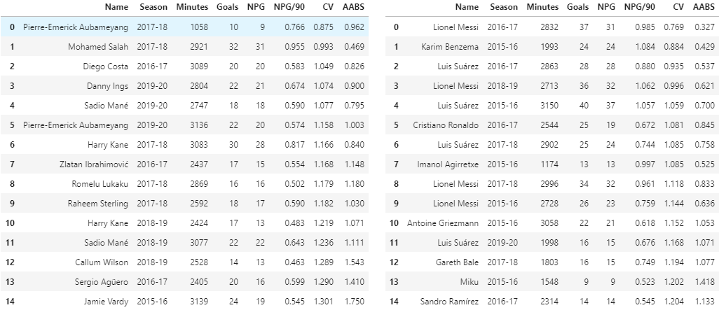
I computed CV and AABS for the top-30 scorers of the Premier League and La Liga from the 2015/16 to the 2019/20 season (all numbers from StatsBomb via FBref). Different seasons are separated too just for comparison purposes, the choice of time range can be flexible. Here’s the top 15 players sorted by CV.
And by AABS.
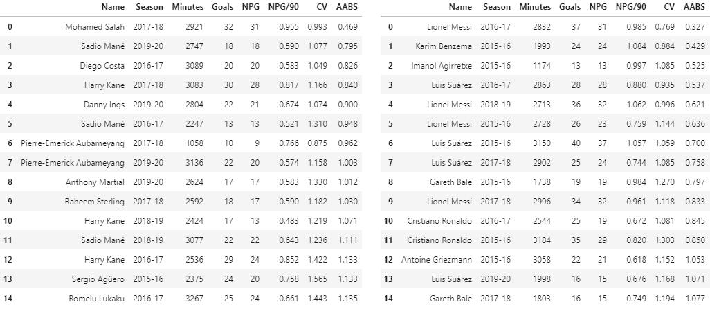
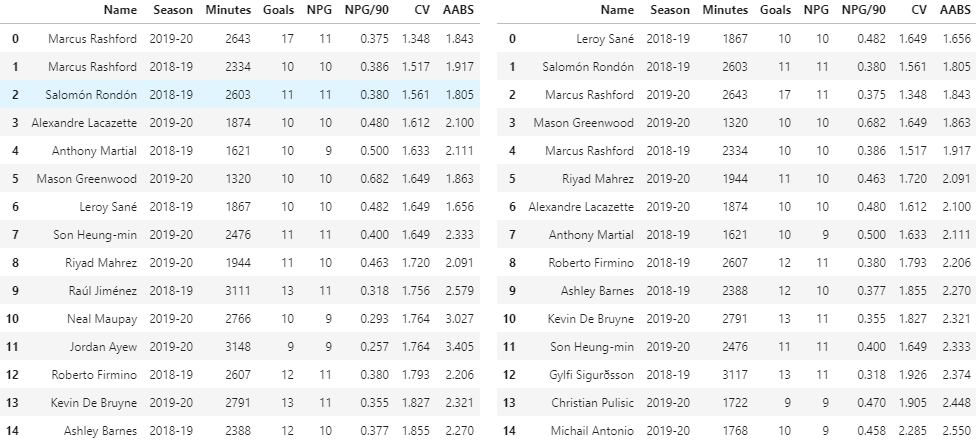
No surprises in some of the top names there such as several Golden Boot/Pichichi winners. Some of the notable ones to me: (1) Callum Wilson’s 2018/19 which ranks 13th in CV, (2) Danny Ing’s superb 2019/20 which features in the top 5 for both metrics, (3) Imanol Agirretxe’s impressive 2015/16 season which unfortunately was cut short due to injury, (4) Ronaldo only appears in the top-15 once for CV. If perhaps you’re not interested in scouting the very best of the best, it is also possible to compare e.g. players with 9-11 NPG from the last 2 PL seasons, where the likes of Salomon Rondon, Neal Maupay and Ashley Barnes appear.
Down memory lane
Now to close the circle with our good friend Dimitar, let’s look at what CV and AABS say about the Premier League Golden Boot winners from the 15 seasons before. Well as expected, Berbatov finds himself at the foot of both tables and thus the least consistent winner. It was also slightly unexpected that Drogba’s 2009/10 topped both tables. Always felt that season doesn’t really get mentioned amongst the best.
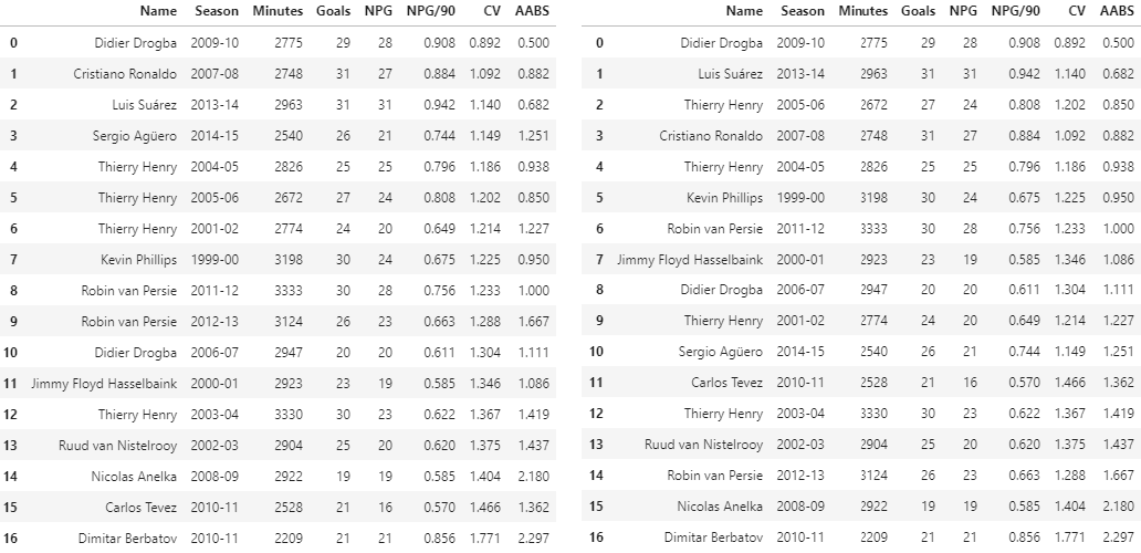
As for La Liga, going back to 1999-00 allows for a peek into the pre Messi-Ronaldo days of greater parity and variety. Messi’s 2012/13 comes out on top again and I won’t bother with further superlatives for him.
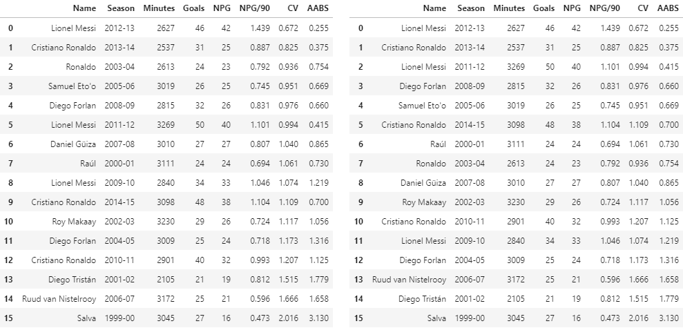

Imagine if 2012/13 Messi didn’t get injured?
Scatter scatter
Lastly, I decided to plot CV vs AABS as a scatter.
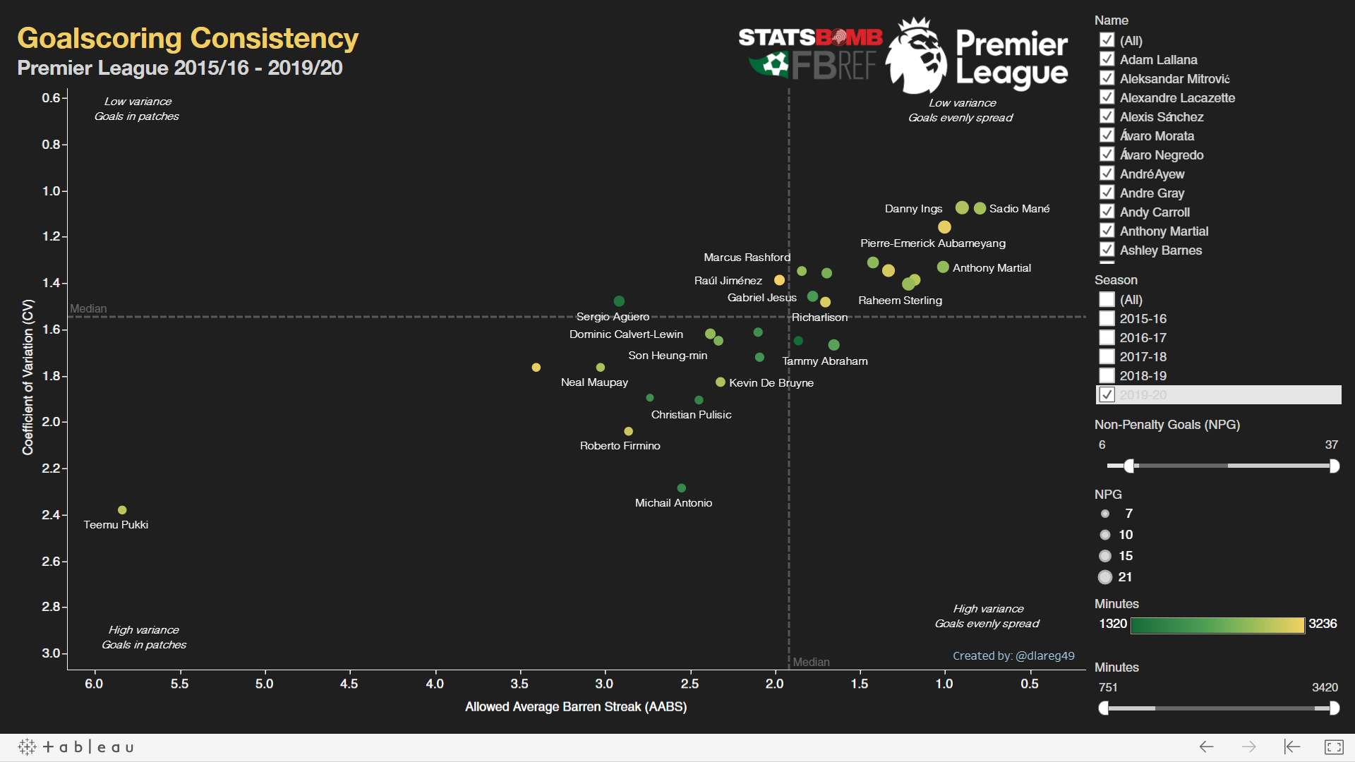
Shouldn’t be a shock that CV and AABS look somewhat correlated, dispersing a little bit at the higher values. For some more fun I’ve made the scatters on Tableau for your own exploration. You can toggle between seasons, NPGs, players to make your own comparisons and such. Have a blast with it :).
Gaps in my defence, and closing off
Looking back at this experiment, the most contentious point might be how I’ve handled the minutes and games inclusion. It is arbitrary, I haven’t thought about a better alternative but I would love to hear your suggestions. Second, the use of the raw NPG may not sit well with the seasoned analytics community as there already are robust underlying performance-related metrics like xG which are better long-term performance predictors. As mentioned earlier a big reason for why I picked NPG was so that I could play around with player comparisons from a much long time period. Hopefully the use of goals also makes this a much more accessible read for visitors who aren’t familiar with xG etc.
I do think though that it’s probably possible to use CV and AABS with xG (or over/underperformance) instead with a few tweaks here and there e.g. setting a xG percentile-based threshold for barren streaks if pronounced temporal fluctuations in xG do occur amongst the data. Maybe extend the time frame beyond a season too for a more accurate picture. All in all, this was largely just a fun exploration for myself over the last week or so, hope you found some interesting things from this too. If you do have any criticisms or suggestions, feel free to contact me via Email or Twitter. Til next time ;)
