Quantifying Player Chemistry - Joint Expected Threat (JxT)
in Football on Football, Premier league, Analytics

Not exactly one from the football commentary hall-off-fame, but devoted Man Utd fans may remember the above words from Rob Hawthorne following Carlos Tevez’s goal to make it 3-1 against Middlesbrough in October 2007 (friendly reminder that Nani scored an absolute banger for 1-0). Tevez’s placed finish followed an intelligent backheel assist from Wayne Rooney, whose situational awareness to draw 3 defenders to him was matched by Tevez’s anticipation of the play. Tevez’s arrival in the summer was met with skepticism over whether the duo could form an effective partnership due to their similar all-action and selfless style. By the end of that season, questions over their chemistry were well and truly put to bed as they, along with Cristiano Ronaldo in a fluid front-three, led Man Utd to the European Double and their most successful season since the millenium.
Player Chemistry I believe, is generally accepted by the football community and fans to exist. Heck, it even is a relatively important thing in Fifa Ultimate Team, where the term is probably most familiar to many.

At the end of my first proper blog post, I mentioned a paper by the team at SciSports who developed a Player Chemistry-quantifying metric using their VAEP framework (Bransen, Van Haaren, 2020). Their paper began with the example of then record signing Andy Carroll and Luis Suarez’s contrasting performances at Liverpool, supporting the notion that signings, regardless of the price tag, are doomed to fail if there’s no chemistry due to a mismatch in playing style. Perhaps more recent examples can further convince you of this occurrence, with Barcelona’s record signings Antoinne Griezzman and Philippe Coutinho performing nowhere near the levels which warranted their purchases so far. As mentioned in Bransen and Van Haaren, despite the importance of player chemistry, this is still a largely overlooked aspect in player evaluation for recruitment purposes, along with existing performance evaluation methods being largely individual-focused (I’m not sure how much this has changed since tbh). Thus, this analysis using JxT represents an attempt to add to the growing work in quantifying player chemistry in football and its uses.
Credit where credit’s due
When I was reading through Bransen and Van Haaren’s derivation of their Player Chemistry metric, I was pleasantly surprised to see the appearance of shared player minutes (which was the topic of my first post) in their formulas, which meant that I could put the numbers I had painstakingly computed to further use, because why not? Hence, a large part of what I’ll describe in the following sections is really just a replication of their work, with the exception of the underlying value metric that’s being used (VAEP in their case). What’s the underlying metric being used here then? You probably could’ve guessed it from the title. That’s right, Expected Threat (xT), a term that should be general knowledge to the football analytics community by now. I won’t elaborate much on xT beyond saying that it is one of several models that value how actions increase or decrease the likelihood of scoring a goal and is often used to quantify player performances. For readers that are new to this term, I defer you to this marvellous write-up and explanation of the xT metric by its creator Karun Singh.
As you’ll see later, most of the heavy lifting has been done by these previous pieces of work, hence the credit really belongs to them. The name of this Player Chemistry metric, Joint Expected Threat (JxT) is also simply the merger of the ‘J’ from Bransen and Van Haaren’s Joint Offensive Impact (JOI) metric and xT.
Deriving JxT
Although my formulation of JxT was originally motivated by JOI, let’s try to derive this from a more fundamental angle and assume we’re starting from scratch. First, we start with the notion that mutual chemistry between players is positively correlated with their performances. From this, we can naturally assume that two players with high mutual chemistry perform better than two players with low mutual chemistry, all other things being equal. Thus, we want a performance metric that measures this joint performance between a player pair. We could use several advanced performance measuring metrics (e.g. xA, key passes) but let’s keep things simple and make use of existing models that assign single-dimensional values to on-the-ball actions anywhere on a football pitch (e.g. xT, g+, PV). Another positive is that these typically operate on event-level data, a good sample size of which is openly available today thanks to the initiatives of Wyscout, Statsbomb and others.
With that in mind, we thus want to formulate a metric that:
Is built on an existing value-attributing base model that operates on event-level data, due to its decent availability compared to e.g. tracking data.
Rewards actions/events (e.g. passes, dribbles) between any two players that contribute to their chemistry. As a starting point let’s term this subset of events “joint interaction actions” between the pair.
Let’s try to gain some intuition for what JxT should look like from event-level data (remember, event-level data only involves actions on the ball, so actions like off-ball runs aren’t logged). I’ll use a ridiculous goal that screams Player Chemistry to me.
Point 2 in the framework requires us to define what constitutes joint interaction actions in event data. We can reasonably first take after the literal meaning of “Joint” and concatenate all events that originate from the two players. Taking Messi and Alves from the above example, that’s simply every event by them. Next, we need to further subset this sequence to contain “Interaction” events. A first logical choice would be the passes between each other. Additionally, we should also consider the immediate events that arise from the preceding exchange (e.g. 1. Messi’s pass to Xavi (after receiving Alves’s pass), 2. Messi’s dribble after receiving Alves’s pass). With event data, these requirements are satisfied by defining an interaction sequence to be consecutive events alternating between the two players. Using these event filters, we can see the events which constitute Messi (M)-Alves (A)’s joint interaction actions to then be something like:
M pass, A pass, M pass, A pass, M pass (to Xavi), M pass, A pass, M pass, A pass, M dribble, M pass, A pass, M shoot (goal).
With our definition of joint interaction actions settled, all that’s left is to select a base model to assign values to each action in the sequence. I’ve chosen xT simply because it’s the first action-value assigning model I came across, although the choice should be quite flexible. Since we’re using xT as the base individual player metric, JxT should also be calculated in a manner faithful to xT (the below may not necessarily apply for a different base metric):
Rewards only ‘successful’ events (passes, dribbles) within an interaction sequence, i.e. moves that were completed without possession being lost.
Rewards actions independent of the end outcome of the possession (i.e. although Messi’s shot is counted as part of the interaction sequence, no reward is assigned to it).
Finally, let’s put everything together into several formulas for better clarity. For a single match m:
where indices i refer to consecutive events alternating between players p and q, ΔxT the change in xT per event and j the index denoting each event sequence as a whole.
JxT for player comparisons
While JxT can be applied for player pairs over single matches up to a season, to enable a fair comparison between pairs who spent different amounts of time on the pitch together within a season, we introduce JxT/90 which weighs total JxT against the pair’s shared minutes:
where min is the total minutes played together per match m.
Comparison with JOI
I mentioned at the start of the above paragraph that my formulation of JxT was originally simply a reapplication of the JOI metric by Bransen and Van Haaren on the xT metric. In some sense while I did try to backwards-engineer the JxT derivation for the benefit of the reader’s intuition, ultimately both methods still share the same underlying principles. The main difference in the xT vs VAEP application for this purpose is that JOI approach rewards VAEP for shot outcomes whereas JxT ignores them. I did experiment with a rough shot rewarding approach by using xT as a proxy for xG but I did not like how it swayed the results quite heavily for strikers.
I’ve seen this somewhere before…
JOI aside, you may have come across a pretty similar concept to this before in several versions of passing networks, e.g.
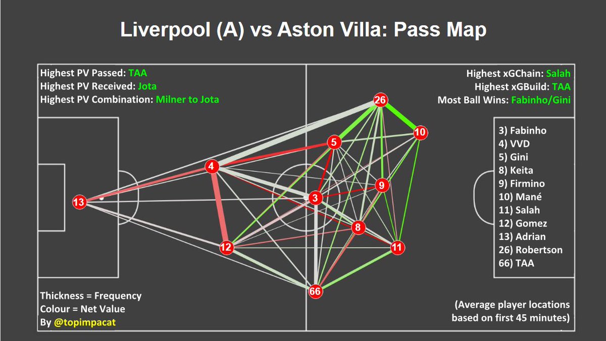
Totally coincidental choice of fixture here
where the edges are coloured according to their strength of the passing link between 2 players. In fact, such visualisations possibly originated from Karun’s idea of interactive passing networks, which assigned directional weights to the edges based on the value from passes given/received values (he was using a version of xT to calculate the values here before he published about xT). While the ideas are indeed quite similar, the main difference is that the joint interaction action sequences don’t only include passes and dribbles between the pair of players.
Observations and Use Cases
With the JxT formula in place, it’s now time to put the metric to test on actual event data and have the resulting player pair JxT values to serve as a sanity check. Following this, several possible applications for JxT in the areas of team selection/evaluation and player recruitment are presented.
The data used for this section are as follows:
Event data used encompasses 5 leagues’ worth of data from the 2017/18 season released as part of Wyscout’s open data initiative. Event-level data constitutes a list of sequential events along with basic attributes for each event, e.g. the player in possession, time elapsed, start and end locations, event outcome etc.
A xT model trained on 2017/18 Premier League data provided by Karun here is used. The original 12x8 grid is then bilinearly interpolated to the Wyscout pitch resolution.
Player minutes data is sourced from Transfermarkt. Note: Transfermarkt does not count added time in the minutes played per game i.e. the max minutes played per match is 90, if a player is subbed on at the 90th, his playing time is logged as 1.
Top JxT Pairs
The table below shows the top 15 players in Europe’s top 5 leagues (Premier League, La Liga, Bundesliga, Serie A, Ligue 1) with the highest cumulative JxT throughout the season (at least 900 minutes together). It shouldn’t be surprising that the #1 pair is De Bruyne-Sterling, with Man City having the most impressive league season that year finishing with a 100 pts. Messi-Suárez are also fairly sensible runner ups, with the duo helping Barcelona to a nearly unbeaten domestic season. Payet-Thauvin were a little surprising to me at first, but I then recalled that Thauvin had a smashing season (22G,14A in 34 in the league) which earned him a call up to the French World Cup squad. Payet himself would’ve been in Russia too if not for an unfortunate injury during the 2018 UEFA Europa League Final.
| Rank | Pair | Team | JxT | Shared Min. |
|---|---|---|---|---|
| 1 | De Bruyne-Sterling | Man City | 4.107 | 2391 |
| 2 | Messi-Suárez | FC Barcelona | 3.889 | 2538 |
| 3 | Payet-Thauvin | Marseille | 3.79 | 2041 |
| 4 | Kessié-Suso | AC Milan | 3.515 | 2696 |
| 5 | Sabaly-Malcom | G. Bordeaux | 3.468 | 2620 |
| 6 | Fàbregas-E. Hazard | Chelsea | 3.34 | 1773 |
| 7 | T. Hazard-Stindl | Bor. M’gladbach | 3.281 | 2633 |
| 8 | Brozović-Perišić | Inter | 3.269 | 1895 |
| 9 | Soares-Tadić | Southampton | 3.256 | 2382 |
| 10 | Hamšík-Insigne | SSC Napoli | 3.249 | 2133 |
| 11 | Eriksen-Kane | Spurs | 3.242 | 2900 |
| 12 | De Bruyne-Silva | Man City | 3.013 | 2216 |
| 13 | Freuler-Gómez | Atalanta | 2.89 | 2465 |
| 14 | Silva-Sterling | Man City | 2.887 | 1796 |
| 15 | Marcelo-Kroos | Real Madrid | 2.83 | 2110 |
On a per 90 basis, the top two from before still appear in the top 15, but we now see the ever-swashbuckling Marcelo in both the first and third spots paired with two other playmakers. In 2nd place is Arsenal’s former focal points of threat creation, both of whom also appeared in the Premier League’s top 15 cumulative xT creators in Karun’s post.
| Rank | Pair | Team | JxT/90 | Shared Min. |
|---|---|---|---|---|
| 1 | Marcelo-Isco | Real Madrid | 0.228 | 1086 |
| 2 | Özil-Sánchez | Arsenal | 0.205 | 1116 |
| 3 | Marcelo-Asensio | Real Madrid | 0.188 | 935 |
| 4 | Fàbregas-Hazard | Chelsea | 0.17 | 1773 |
| 5 | Payet-Thauvin | Marseille | 0.167 | 2041 |
| 6 | Brozović-Perišić | Inter | 0.155 | 1895 |
| 7 | De Bruyne-Sterling | Man City | 0.155 | 2391 |
| 8 | Kolarov-Perotti | AS Roma | 0.154 | 1523 |
| 9 | Iniesta-Messi | FC Barcelona | 0.15 | 1599 |
| 10 | Ramos-Marcelo | Real Madrid | 0.146 | 1404 |
| 11 | D. Silva-Sterling | Man City | 0.145 | 1796 |
| 12 | López-Thauvin | Marseille | 0.139 | 1115 |
| 13 | Schulz-Kramarić | TSG Hoffenheim | 0.139 | 1307 |
| 14 | Messi-Suárez | FC Barcelona | 0.138 | 2538 |
| 15 | Hamšík-Insigne | SSC Napoli | 0.137 | 2133 |
Analysing team chemistry through JxT Networks
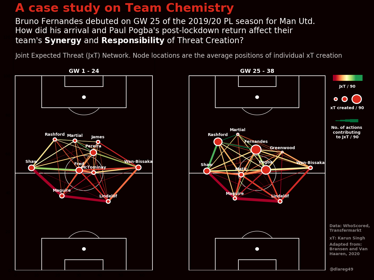
JxT data can also be used to depict team chemistry over single or multiple matches via network analysis. By complimenting player pair JxT values with individual xT values; average xT creating positions and the number of JxT creating actions per pair, JxT networks visualise where the hubs of xT creation and strongest JxT links are in a team in a manner similar to passing networks. In my first post on Twitter with this visualisation, I depicted how Man Utd’s productivity and chemistry, especially in midfield, improved over the 2019/20 season after the arrival of Bruno Fernandes and subsequent return of Paul Pogba.
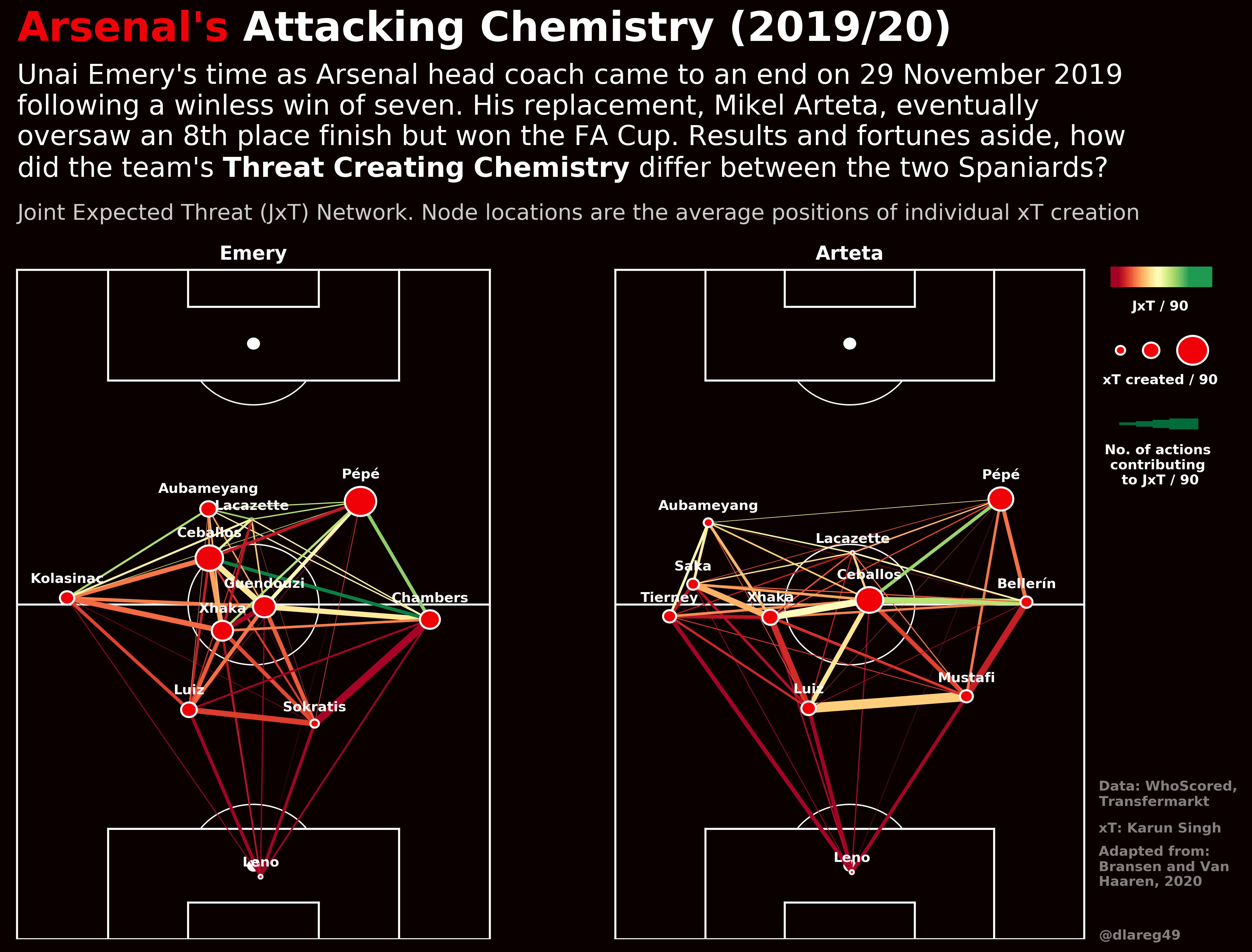
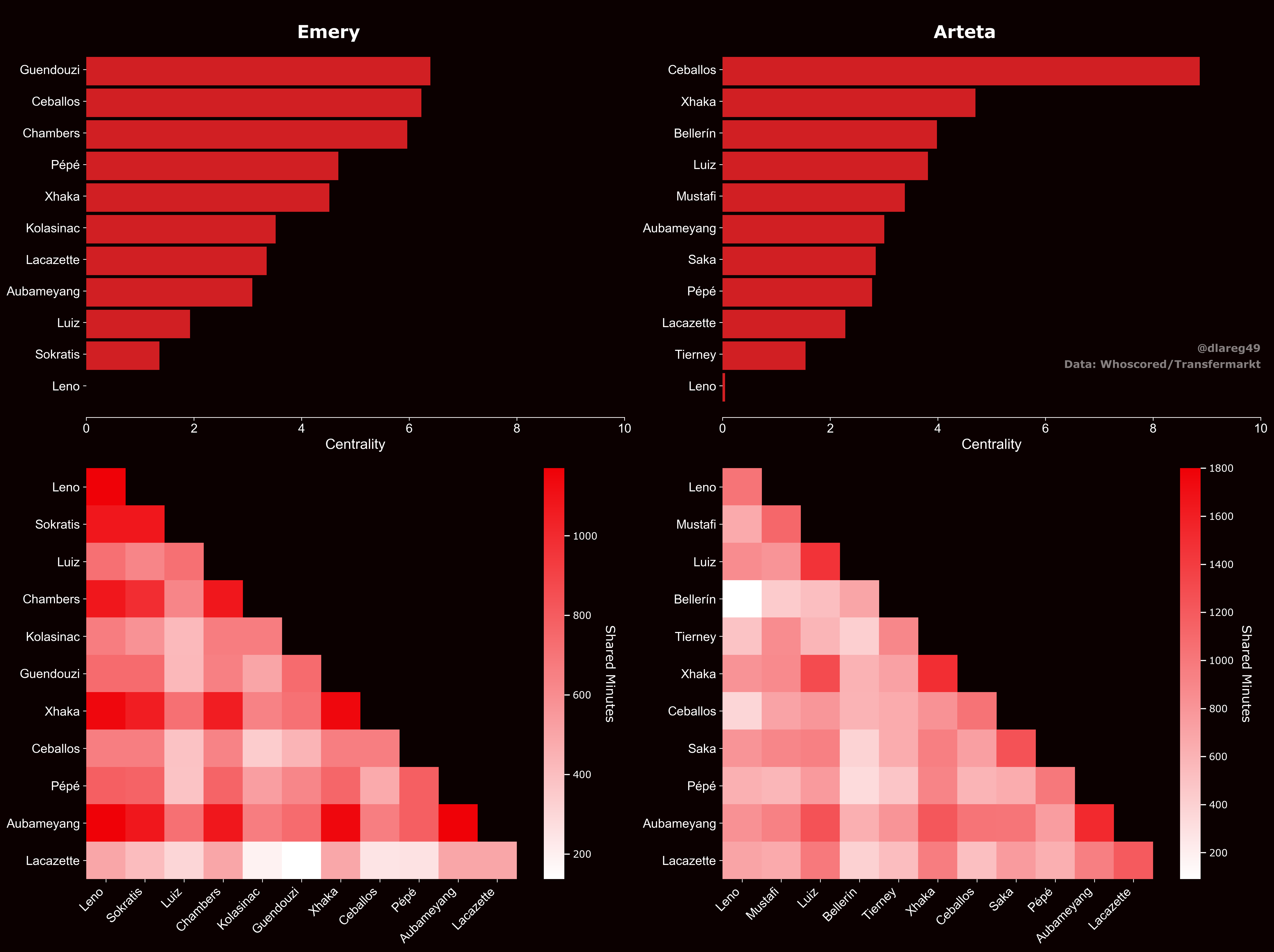
My second case study with this method looked at Arsenal’s JxT networks under Emery and Arteta in the 2019/20 league season. These showed that the changes were largely in Arsenal’s shape and attacking structure, whereas xT and JxT did not seem to differ much (if anything they seemed to create xT better under Emery). The data was also used to compute network centrality in terms of total JxT volume, which depicted Ceballos as being the hub under both managers, as well as a shared minutes matrix which showed how many minutes were shared between each selected eleven.
Beyond this, the analysis can be extended to the whole squad of the team to assemble a maximum-chemistry starting eleven and perhaps even identify the best substitutes to bring on based on a least chemistry reduced rule. Bransen and Van Haaren explored this in their paper in section 5.
Predicting JxT/90 for player recruitment
Another idea from the Player Chemistry paper that I’m still in the process of emulating is to apply JxT/90 for player recruitment purposes. Being able to predict how well any two players will play together can be a powerful tool. Although JxT/90 values between players that have never played together don’t exist, machine learning regression models offer us a tool for predicting hypothetical JxT/90 values. This is achieved by using player characteristics or statistics that are likely to influence chemistry as predictors in the feature engineering.
Since Bransen and Van Haaren reported that player role-based characteristics were particularly impactful (in contrast to cultural features), as a first guess (and also for convenience), I used the same features (2017/18 player stats from FBref) that Parth Arthale used in his PCA model to derive distinct playing styles and player similarity scores as the predictors. Each player (with at least 1000 minutes played) pair’s feature vector consisted of the mean and absolute difference of their respective features (i.e. for 112 features per player = 224 per pair). The dataset was then split into training (La Liga, Bundesliga, Serie A, Ligue 1), validation (10 Premier League teams) and test (remaining 10 Premier League teams) sets.
The XGBoost algorithm was used to train the regression model, with hyperparameters tuned on the validation set to optimise the validation RMSE. Against a naive baseline model which predicts JxT/90 to always be the average training set value with RMSE of 0.0263 on the test set, the trained model obtained a lower RMSE of 0.01802.
While the architecture of this model can definitely be improved, let’s consider some use cases for it. Say Barcelona who were interested in procuring Antoinne Griezmann after the 2017/18 season would also like to consider alternatives in case the move fell through. Barca’s recruitment team could use this model to predict JxT/90 between their candidates and certain members of the squad that would play in close proximity to them. The figure below depicts predicted JxT/90 between several shortlisted players and prominent Barca midfielders and forwards. We see that the model predicts that Griezmann’s isn’t really the optimal choice for Barcelona chemistry-wise.
The question could also be flipped around for a scenario e.g. say Riyad Mahrez’s agent/agency who were looking for his big summer move in 2018 could’ve consulted such a tool to add a further dimension to identifying suitable clubs for him. While these two examples consider select teammates with which the predictions are made, the method can always be tweaked around to consider e.g. the method can always be tweaked around to consider e.g. overall lineups that would maximise overall JxT/90 with the player in focus.
Closing Thoughts
One important aspect of chemistry that I’ve omitted so far is of course, the defensive side of it. If a club’s in the market for a centre-back to bolster their deference, surely a defense-oriented chemistry metric would take precedence over JxT. While this is something that Bransen and Van Haaren have modelled in their paper (see Joint Defensive Impact (JDI)), due to event data constraints the metric is something that’s more inferred rather than directly measured. I’ve not decided how to go about implementing this with xT yet, perhaps this is something that needs a little more care and could use the help of tracking data.
That aside, I’d like to empathise that JxT, like xT and many other similar models, are by no means perfect and understanding the results with context is always important. For instance, perhaps Griezmann could be unfavourably scored by JxT as metrics like xG (and I suppose xT too) tend to portray counter-attacking teams poorly (as such teams would have fewer ball actions then average). Would a possession adjusted score maybe give a fairer reflection? Or is it fair to tinker with the raw score in the first place? Additionally, the predictive model and the predictions made above relied on just a season’s worth of data. I’d think clubs typically consider a longer time horizon than that. Last but not least, the JxT metric is purely performance-based, but performances aren’t solely dependent on the players themselves. Tactics, the manager, overall team quality are just some factors that influence performance. Thus, a truly accurate picture of player chemistry is really complicated and just like football analytics as a whole, there will be more to explore.